Writing a log, dumping data, looking for file to be used in Bulk insert…

There are many situations when you would want to have access to files from inside your SQL code on Microsoft SQL Server.

Did you know that you actually can do this? No? Check below for code snippets to perform various operations on files. It is presented in form of the functions but you are actually not limited to that

Prerequisites and assumptions

1. Your script should have sufficient rights to perform required access to files (not necessarily local).
2. Scripting.FileSystemObject should be present at your SQL Server location and accessible.

Check if file exists

Write string into file

Read File As Table

Enjoy.

https://blog.dragonsoft.us/2008/02/15/sql-manage-files-from-inside-sql-code/

udayarumilli.com/script-to-monitor-sql-server-memory-usage/

Introduction:

This post will takes you through the T-SQL Script to monitor SQL Server Memory Usage. In previous blog post we have explained the parameters involved in understanding sql server memory usage. There are total 7 scripts to monitor SQL Server Memory Usage.

• Buffer Pool Usage
• System Memory Information
• SQL Server Process Memory Usage Information
• Buffer Usage by Database
• Object Wise Buffer Usage
• Top 25 Costliest Stored Procedures – Logical Reads
• Top Performance Counters

Script to Monitor SQL Server Memory Usage: Buffer Pool Usage

Results:

BPool_Committed_MB: Actual memory committed/used by the process (SQL Server).

BPool_Commit_Tgt_MB: Actual memory SQL Server tried to consume.

BPool_Visible_MB: Number of 8-KB buffers in the buffer pool that are directly accessible in the process virtual address space (SQL Server VAS).

Analysis:

BPool_Commit_Tgt_MB > BPool_Committed_MB: SQL Server Memory Manager tries to obtain additional memory

BPool_Commit_Tgt_MB < BPool_Committed_MB: SQL Server Memory Manager tries to shrink the amount of memory committed

If the value of BPool_Visible_MB is too low: We might receive out of memory errors or memory dump will be created.

Script to Monitor SQL Server Memory Usage: System Memory Information

Results:

total_physical_memory_mb: Actual Physical Memory installed in OS

available_physical_memory_mb: Available Physical Memory

total_page_file_mb: Pagefile size on OS

available_page_file_mb: Available page file size

Percentage_Used: Physical Memory Percentage used

system_memory_state_desc: Memory current Health status

Analysis:

available_physical_memory_mb: Should be some positive sign based on total physical memory

available_page_file_mb: Should be some positive sign based on your total page file

Percentage_Used: 100% for a long time indicates a memory pressure

system_memory_state_desc: should be Available physical memory is high / steady

Script to Monitor SQL Server Memory Usage: SQL Server Process Memory Usage

Results:

physical_memory_in_use: Indicates the process working set in KB, as reported by operating system, as well as tracked allocations by using large page APIs

locked_page_allocations: Specifies memory pages locked in memory

virtual_address_space_committed: Indicates the amount of reserved virtual address space that has been committed or mapped to physical pages.

available_commit_limit: Indicates the amount of memory that is available to be committed by the process (SQL server)

page_fault_count: Indicates the number of page faults that are incurred by the SQL Server process

Analysis:

physical_memory_in_use: We can’t figure out the exact amount of physical memory using by sqlservr.exe using task manager but this column showcase the actual amount of physical memory using by SQL Server.

locked_page_allocations: If this is > 0 means Locked Pages is enabled for SQL Server which is one of the best practice

available_commit_limit: This indciates the available amount of memory that can be committed by the process sqlservr.exe

page_fault_count: Pages fetching from the page file on the hard disk instead of from physical memory. Consistently high number of hard faults per second represents Memory pressure.

Script to Monitor SQL Server Memory Usage: Database Wise Buffer Usage

Results:

db_name: Name of the database in the given SQL server Instance

db_buffer_pages: Total number of corresponding database pages that are in buffer pool

db_buffer_Used_MB: Database wise Buffer size used in MB

db_buffer_Free_MB: Database wise Buffer Size Free (sum of free space on all pages) in MB.

db_buffer_percent: Database wise percentage of Buffer Pool usage

Analysis:

We can quickly find out the top databases which are consuming more Memory / Buffer Pool from the given SQL server Instance

Script to Monitor SQL Server Memory Usage: Object Wise Buffer Usage

Results:

Object: Name of the Object

Type: Type of the object Ex: USER_TABLE

Index: Name of the Index

Index_Type: Type of the Index “Clustered / Non Clustered / HEAP” etc

buffer_pages: Object wise number of pages is in buffer pool

buffer_mb: Object wise buffer usage in MB

Analysis:

From the previous script we can get the top databases using memory. This script helps you out in finding the top objects that are using the buffer pool. Top objects will tell you the objects which are using the major portion of the buffer pool.If you find anything suspicious then you can dig into it.

Script to Monitor SQL Server Memory Usage: Top 25 Costliest Stored Procedures by Logical Reads

Results:

SP Name: Stored Procedure Name

TotalLogicalReads: Total Number of Logical Reads since this stored procedure was last compiled

AvgLogicalReads: Average Number of Logical Reads since this stored procedure was last compiled

execution_count: Number of Times SP got executed since it was compiled

total_elapsed_time: Total elapsed time for this proc since last time compiled

avg_elapsed_time: Average elapsed time

cached_time: Time at which the stored procedure was added to the cache.

Analysis:

• This helps you find the most expensive cached stored procedures from a memory perspective
• You should look at this if you see signs of memory pressure
• More number of logical reads means you need to check execution plan to find the bottleneck

Script to Monitor SQL Server Memory Usage: Top Performance Counters – Memory

Results:

Total Server Memory: Shows how much memory SQL Server is using. The primary use of SQL Server’s memory is for the buffer pool, but some memory is also used for storing query plans and keeping track of user process information.

Target Server Memory: This value shows how much memory SQL Server attempts to acquire. If you haven’t configured a max server memory value for SQL Server, the target amount of memory will be about 5MB less than the total available system memory.

Connection Memory (GB): The Connection Memory specifies the total amount of dynamic memory the server is using for maintaining connections

Lock Memory (GB): Shows the total amount of memory the server is using for locks

SQL Cache Memory: Total memory reserved for dynamic SQL statements.

Optimizer Memory: Memory reserved for query optimization.

Granted Workspace Memory: Total amount of memory currently granted to executing processes such as hash, sort, bulk copy, and index creation operations.

Cursor memory usage: Memory using for cursors

Free pages: Amount of free space in pages which are commited but not currently using by SQL Server

Reserved Pages: Shows the number of buffer pool reserved pages.

Stolen pages (MB): Memory used by SQL Server but not for Database pages.It is used for sorting or hashing operations, or “as a generic memory store for allocations to store internal data structures such as locks, transaction context, and connection information.

Cache Pages: Number of 8KB pages in cache.

Page life expectancy: Average how long each data page is staying in buffer cache before being flushed out to make room for other pages

Free list stalls / sec: Number of times a request for a “free” page had to wait for one to become available.

Checkpoint Pages/sec: Checkpoint Pages/sec shows the number of pages that are moved from buffer to disk per second during a checkpoint process

Lazy writes / sec: How many times per second lazy writer has to flush dirty pages out of the buffer cache instead of waiting on a checkpoint.

Memory Grants Outstanding: Number of processes that have successfully acquired workspace memory grant.

Memory Grants Pending: Number of processes waiting on a workspace memory grant.

process_physical_memory_low: Process is responding to low physical memory notification

process_virtual_memory_low: Indicates that low virtual memory condition has been detected

Min Server Memory: Minimum amount of memory SQL Server should acquire

Max Server Memory: Maximum memory that SQL Server can acquire from OS

Buffer cache hit ratio: Percentage of pages that were found in the buffer pool without having to incur a read from disk.

Analysis:

Total Server Memory is almost same as Target Server Memory: Good Health

Total Server Memory is much smaller than Target Server Memory: There is a Memory Pressure or Max Server Memory is set to too low.

Connection Memory: When high, check the number of user connections and make sure it’s under expected value as per your business

Optimizer Memory: Ideally, the value should remain relatively static. If this isn’t the case you might be using dynamic SQL execution excessively.

Higher the value for Stolen Pages: Find the costly queries / procs and tune them

Higher the value for Checkpoint Pages/sec: Problem with I/O, Do not depend on Automatic Checkpoints and use In-direct checkpoints.

Page life expectancy: Usually 300 to 400 sec for each 4 GB of memory. Lesser the value means memory pressure

Free list stalls / sec: High value indicates that the server could use additional memory.

Memory Grants Outstanding: Higher value indicates peak user activity

Memory Grants Pending: Higher value indicates SQL Server need more memory

process_physical_memory_low & process_virtual_memory_low: Both are equals to 0 means no internal memory pressure

Min Server Memory: If it is 0 means default value didnt get changed, it’ll always be better to have a minimum amount of memory allocated to SQL Server

Max Server Memory: If it is default to 2147483647, change the value with the correct amount of memory that you can allow SQL Server to utilize.

Buffer cache hit ratio: This ratio should be in between 95 and 100. Lesser value indicates memory pressure

Script to Monitor SQL Server Memory Usage: DBCC MEMORYSTATUS

Finally DBCC MemoryStatus:

• It gives as much as memory usage information based on object wise / component wise.
• First table gives us the complete details of server and process memory usage details and memory alert indicators.
• We can also get memory usage by buffer cache, Service Broker, Temp tables, Procedure Cache, Full Text, XML, Memory Pool Manager, Audit Buffer, SQLCLR, Optimizer, SQLUtilities, Connection Pool etc.

Summary:

These Scripts will help you in understanding the current memory usage by SQL Server. To maintain a healthy database management system:

• Monitor the system for few business days in peak hours and fix the baselines
• Identify the correct required configurations for your database server and make the required changes
• Identify top 10 queries / procedures based on Memory and CPU usage
• Fine tune these top 10 queries / procedures

Note:

These scripts are tested on SQL Server 2008, 2008 R2, 2012 and 2014. As we always suggests please test these scripts on Dev/Test environment before using them on production systems.

References:

Would like to thank famous MVPs / MCM / bloggers (Glenn Berry, Brent Ozar, Jonathan Kehayias, John Sansom) for the tremendous explanation on sql server internals. Their articles are very informative and helpful in understanding SQL Server internals.

Also Check:

SQL Server Memory Usage

SQL Server CPU Utilization

Those who have been working with SQL Server administration for a while now undoubtedly have at times referred to the old SQL Server system tables in order to automate some processes, or document their tables by for example combining the sysobjects and syscolumns tables. As per SQL Server 2005 and onwards, Microsoft added a number of Dynamic Management Views (DMV) that take simplify all kinds of management tasks.

List of SQL Server 2000 system tables and their 2005 equivalent management views, as well as a brief description what kind of information to find in the views.

Dynamic Management Views existing in the Master database

Dynamic Management Views existing in every database.

原文：Script to retrieve SQL Server database backup history and no backups

Problem

There is a multitude of data to be mined from within the Microsoft SQL Server system views. This data is used to present information back to the end user of the SQL Server Management Studio (SSMS) and all third party management tools that are available for SQL Server Professionals. Be it database backup information, file statistics, indexing information, or one of the thousands of other metrics that the instance maintains, this data is readily available for direct querying and assimilation into your “home-grown” monitoring solutions as well. This tip focuses on that first metric: database backup information. Where it resides, how it is structured, and what data is available to be mined.

Solution

The msdb system database is the primary repository for storage of SQL Agent, backup, Service Broker, Database Mail, Log Shipping, restore, and maintenance plan metadata. We will be focusing on the handful of system views associated with database backups for this tip:

• dbo.backupset: provides information concerning the most-granular details of the backup process
• dbo.backupmediafamily: provides metadata for the physical backup files as they relate to backup sets
• dbo.backupfile: this system view provides the most-granular information for the physical backup files

Based upon these tables, we can create a variety of queries to collect a detailed insight into the status of backups for the databases in any given SQL Server instance.

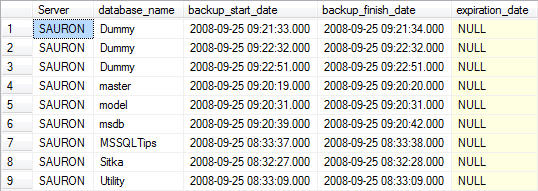
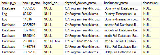
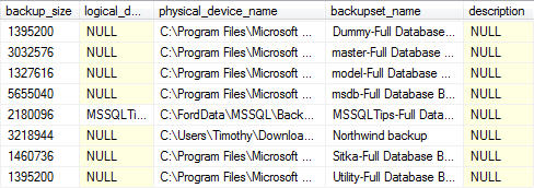
Database Backups for all databases For Previous Week

--------------------------------------------------------------------------------- 
--Database Backups for all databases For Previous Week 
--------------------------------------------------------------------------------- 
SELECT 
CONVERT(CHAR(100), SERVERPROPERTY('Servername')) AS Server, 
msdb.dbo.backupset.database_name, 
msdb.dbo.backupset.backup_start_date, 
msdb.dbo.backupset.backup_finish_date, 
msdb.dbo.backupset.expiration_date, 
CASE msdb..backupset.type 
WHEN 'D' THEN 'Database' 
WHEN 'L' THEN 'Log' 
END AS backup_type, 
msdb.dbo.backupset.backup_size, 
msdb.dbo.backupmediafamily.logical_device_name, 
msdb.dbo.backupmediafamily.physical_device_name, 
msdb.dbo.backupset.name AS backupset_name, 
msdb.dbo.backupset.description 
FROM msdb.dbo.backupmediafamily 
INNER JOIN msdb.dbo.backupset ON msdb.dbo.backupmediafamily.media_set_id = msdb.dbo.backupset.media_set_id 
WHERE (CONVERT(datetime, msdb.dbo.backupset.backup_start_date, 102) >= GETDATE() - 7) 
ORDER BY 
msdb.dbo.backupset.database_name, 
msdb.dbo.backupset.backup_finish_date

Note: for readability the output was split into two screenshots.

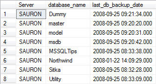
Most Recent Database Backup for Each Database

------------------------------------------------------------------------------------------- 
--Most Recent Database Backup for Each Database 
------------------------------------------------------------------------------------------- 
SELECT  
   CONVERT(CHAR(100), SERVERPROPERTY('Servername')) AS Server, 
   msdb.dbo.backupset.database_name,  
   MAX(msdb.dbo.backupset.backup_finish_date) AS last_db_backup_date 
FROM   msdb.dbo.backupmediafamily  
   INNER JOIN msdb.dbo.backupset ON msdb.dbo.backupmediafamily.media_set_id = msdb.dbo.backupset.media_set_id  
WHERE  msdb..backupset.type = 'D' 
GROUP BY 
   msdb.dbo.backupset.database_name  
ORDER BY  
   msdb.dbo.backupset.database_name 

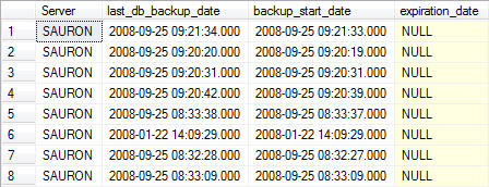
Most Recent Database Backup for Each Database – Detailed

You can join the two result sets together by using the following query in order to return more detailed information about the last database backup for each database. The LEFT JOIN allows you to match up grouped data with the detailed data from the previous query without having to include the fields you do not wish to group on in the query itself.

------------------------------------------------------------------------------------------- 
--Most Recent Database Backup for Each Database - Detailed 
------------------------------------------------------------------------------------------- 
SELECT  
   A.[Server],  
   A.last_db_backup_date,  
   B.backup_start_date,  
   B.expiration_date, 
   B.backup_size,  
   B.logical_device_name,  
   B.physical_device_name,   
   B.backupset_name, 
   B.description 
FROM 
   ( 
   SELECT   
       CONVERT(CHAR(100), SERVERPROPERTY('Servername')) AS Server, 
       msdb.dbo.backupset.database_name,  
       MAX(msdb.dbo.backupset.backup_finish_date) AS last_db_backup_date 
   FROM    msdb.dbo.backupmediafamily  
       INNER JOIN msdb.dbo.backupset ON msdb.dbo.backupmediafamily.media_set_id = msdb.dbo.backupset.media_set_id  
   WHERE   msdb..backupset.type = 'D' 
   GROUP BY 
       msdb.dbo.backupset.database_name  
   ) AS A 
    
   LEFT JOIN  

   ( 
   SELECT   
   CONVERT(CHAR(100), SERVERPROPERTY('Servername')) AS Server, 
   msdb.dbo.backupset.database_name,  
   msdb.dbo.backupset.backup_start_date,  
   msdb.dbo.backupset.backup_finish_date, 
   msdb.dbo.backupset.expiration_date, 
   msdb.dbo.backupset.backup_size,  
   msdb.dbo.backupmediafamily.logical_device_name,  
   msdb.dbo.backupmediafamily.physical_device_name,   
   msdb.dbo.backupset.name AS backupset_name, 
   msdb.dbo.backupset.description 
FROM   msdb.dbo.backupmediafamily  
   INNER JOIN msdb.dbo.backupset ON msdb.dbo.backupmediafamily.media_set_id = msdb.dbo.backupset.media_set_id  
WHERE  msdb..backupset.type = 'D' 
   ) AS B 
   ON A.[server] = B.[server] AND A.[database_name] = B.[database_name] AND A.[last_db_backup_date] = B.[backup_finish_date] 
ORDER BY  
   A.database_name

Note: for readability the output was split into two screenshots.

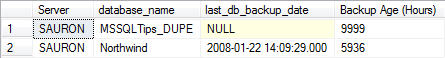
Databases Missing a Data (aka Full) Back-Up Within Past 24 Hours

At this point we’ve seen how to look at the history for databases that have been backed up. While this information is important, there is an aspect to backup metadata that is slightly more important – which of the databases you administer have not been getting backed up. The following query provides you with that information (with some caveats.)

------------------------------------------------------------------------------------------- 
--Databases Missing a Data (aka Full) Back-Up Within Past 24 Hours 
------------------------------------------------------------------------------------------- 
--Databases with data backup over 24 hours old 
SELECT 
   CONVERT(CHAR(100), SERVERPROPERTY('Servername')) AS Server, 
   msdb.dbo.backupset.database_name, 
   MAX(msdb.dbo.backupset.backup_finish_date) AS last_db_backup_date, 
   DATEDIFF(hh, MAX(msdb.dbo.backupset.backup_finish_date), GETDATE()) AS [Backup Age (Hours)] 
FROM    msdb.dbo.backupset 
WHERE     msdb.dbo.backupset.type = 'D'  
GROUP BY msdb.dbo.backupset.database_name 
HAVING      (MAX(msdb.dbo.backupset.backup_finish_date) < DATEADD(hh, - 24, GETDATE()))  

UNION  

--Databases without any backup history 
SELECT      
   CONVERT(CHAR(100), SERVERPROPERTY('Servername')) AS Server,  
   master.dbo.sysdatabases.NAME AS database_name,  
   NULL AS [Last Data Backup Date],  
   9999 AS [Backup Age (Hours)]  
FROM 
   master.dbo.sysdatabases LEFT JOIN msdb.dbo.backupset 
       ON master.dbo.sysdatabases.name  = msdb.dbo.backupset.database_name 
WHERE msdb.dbo.backupset.database_name IS NULL AND master.dbo.sysdatabases.name <> 'tempdb' 
ORDER BY  
   msdb.dbo.backupset.database_name

Now let me explain those caveats, and this query. The first part of the query returns all records where the last database (full) backup is older than 24 hours from the current system date. This data is then combined via the UNION statement to the second portion of the query. That second statement returns information on all databases that have no backup history. I’ve taken the liberty of singling tempdb out from the result set since you do not back up that system database. It is recreated each time the SQL Server services are restarted. That is caveat #1. Caveat #2 is the arbitrary value I’ve assigned to the aging value for databases without any backup history. I’ve set that value at 9999 hours because in my environment I want to place a higher emphasis on those databases that have never been backed up.

原文地址：http://www.sqlservercentral.com/articles/SSMS/160267/?utm_source=SSC&utm_medium=pubemail

By Konstantin Taranov, 2017/08/14

CREATE TABLE TestData(ID INT IDENTITY (1,1), CreatedDate DATETIME)
GO

INSERT INTO TestData(CreatedDate) SELECT GetDate()
GO 10

ConnectRetryCount=0

EXEC sp_addextendedproperty
@name = N'microsoft_database_tools_support',
@value = 'Hide',
@level0type = N'Schema', @level0name = 'Person',
@level1type = N'Table', @level1name = 'Address';
GO

EXEC sp_dropextendedproperty
@name = N'microsoft_database_tools_support',
@level0type = N'Schema', @level0name = 'Person',
@level1type = N'Table', @level1name = 'Address';
GO

DENY VIEW DEFINITION ON Schema.Table TO UserName;

"C:\Program Files (x86)\Microsoft SQL Server\140\Tools\Binn\ManagementStudio\Ssms.exe" "C:\Users\taranov\Documents\SQL Server Management Studio\Projects\MySQLServerScripts.ssmssln" -nosplash

C:\Program Files (x86)\Microsoft SQL Server\[140|130|120|110]\Tools\Binn\ ManagementStudio\SqlWorkbenchProjectItems\Sql\SQLFile.sql

BEGIN TRANSACTION;
 
 
-- COMMIT   TRANSACTION;
-- ROLLBACK TRANSACTION;

/***************************************************************
  Author: John Morehouse
  Summary: This script display what SET options are enabled for the current session.
 
  You may alter this code for your own purposes. You may republish altered code as long as you give due credit.
 
  THIS CODE AND INFORMATION IS PROVIDED "AS IS" WITHOUT WARRANTY OF ANY KIND, EITHER EXPRESSED OR IMPLIED, INCLUDING BUT NOT LIMITED TO THE IMPLIED WARRANTIES OF MERCHANTABILITY AND/OR FITNESS FOR A PARTICULAR PURPOSE.
***************************************************************/
SELECT 'Disable_Def_Cnst_Chk'    AS 'Option', CASE @@options & 1     WHEN 0 THEN 0 ELSE 1 END AS 'Enabled/Disabled' UNION ALL
SELECT 'IMPLICIT_TRANSACTIONS'   AS 'Option', CASE @@options & 2     WHEN 0 THEN 0 ELSE 1 END AS 'Enabled/Disabled' UNION ALL
SELECT 'CURSOR_CLOSE_ON_COMMIT'  AS 'Option', CASE @@options & 4     WHEN 0 THEN 0 ELSE 1 END AS 'Enabled/Disabled' UNION ALL
SELECT 'ANSI_WARNINGS'           AS 'Option', CASE @@options & 8     WHEN 0 THEN 0 ELSE 1 END AS 'Enabled/Disabled' UNION ALL
SELECT 'ANSI_PADDING'            AS 'Option', CASE @@options & 16    WHEN 0 THEN 0 ELSE 1 END AS 'Enabled/Disabled' UNION ALL
SELECT 'ANSI_NULLS'              AS 'Option', CASE @@options & 32    WHEN 0 THEN 0 ELSE 1 END AS 'Enabled/Disabled' UNION ALL
SELECT 'ARITHABORT'              AS 'Option', CASE @@options & 64    WHEN 0 THEN 0 ELSE 1 END AS 'Enabled/Disabled' UNION ALL
SELECT 'ARITHIGNORE'             AS 'Option', CASE @@options & 128   WHEN 0 THEN 0 ELSE 1 END AS 'Enabled/Disabled' UNION ALL
SELECT 'QUOTED_IDENTIFIER'       AS 'Option', CASE @@options & 256   WHEN 0 THEN 0 ELSE 1 END AS 'Enabled/Disabled' UNION ALL
SELECT 'NOCOUNT'                 AS 'Option', CASE @@options & 512   WHEN 0 THEN 0 ELSE 1 END AS 'Enabled/Disabled' UNION ALL
SELECT 'ANSI_NULL_DFLT_ON'       AS 'Option', CASE @@options & 1024  WHEN 0 THEN 0 ELSE 1 END AS 'Enabled/Disabled' UNION ALL
SELECT 'ANSI_NULL_DFLT_OFF'      AS 'Option', CASE @@options & 2048  WHEN 0 THEN 0 ELSE 1 END AS 'Enabled/Disabled' UNION ALL
SELECT 'CONCAT_NULL_YIELDS_NULL' AS 'Option', CASE @@options & 4096  WHEN 0 THEN 0 ELSE 1 END AS 'Enabled/Disabled' UNION ALL
SELECT 'NUMERIC_ROUNDABORT'      AS 'Option', CASE @@options & 8192  WHEN 0 THEN 0 ELSE 1 END AS 'Enabled/Disabled' UNION ALL
SELECT 'XACT_ABORT'              AS 'Option', CASE @@options & 16384 WHEN 0 THEN 0 ELSE 1 END AS 'Enabled/Disabled';

常用DBCC命令详解

Transact-SQL 编程语言提供 DBCC 语句作为 SQL Server 的数据库控制台命令。

DBCC 命令使用输入参数并返回值。所有 DBCC 命令参数都可以接受 Unicode 和 DBCS 文字。
维护命令
1、DBCC INPUTBUFFER
功能：显示从客户端发送到 Microsoft SQL Server实例的最后一个语句。
格式：DBCC INPUTBUFFER ( session_id [ , request_id ] )[WITH NO_INFOMSGS ]
执行权限：用户必须是 sysadmin 固定服务器角色的成员。
用户必须具有 VIEW SERVER STATE 权限。
相关命令：SELECT @@spid
SELECT request_id FROM sys.dm_exec_requests WHERE session_id = @@spid

2、DBCC OUTPUTBUFFER
功能：以十六进制和 ASCII 格式返回指定 session_id 的当前输出缓冲区。
格式：DBCC OUTPUTBUFFER ( session_id [ , request_id ] )[ WITH NO_INFOMSGS ]
执行权限：用户必须是 sysadmin 固定服务器角色的成员。
相关命令：SELECT @@spid
SELECT request_id FROM sys.dm_exec_requests WHERE session_id = @@spid

3、DBCC SHOWCONTIG
功能：显示指定的表或视图的数据和索引的碎片信息。
格式：DBCC SHOWCONTIG [ (对象名) ]
[ WITH  { [ , [ ALL_INDEXES ] ] [ , [ TABLERESULTS ] ] [ , [ FAST ] ] [ , [ ALL_LEVELS ] ]  [ NO_INFOMSGS ] } ]
执行权限：用户必须是对象所有者，或是 sysadmin 固定服务器角色、db_owner 固定数据库角色或 db_ddladmin 固定数据库角色的成员。
例：DBCC SHOWCONTIG (‘TableName’)
说明：可使用DBCC SHOWCONTIG 和 DBCC INDEXDEFRAG 对数据库中的索引进行碎片整理

4、DBCC OPENTRAN
功能：如果在指定数据库内存在最早的活动事务和最早的分布式和非分布式复制事务，则显示与之有关的信息。
格式：DBCC OPENTRAN [ ( [ database_name | database_id | 0 ] ) ]
{ [ WITH TABLERESULTS ] [ , [ NO_INFOMSGS ] ] }]
例：DBCC OPENTRAN (DataBaseName) WITH TABLERESULTS

5、DBCC SQLPERF
功能：为所有数据库提供事务日志空间用法的统计信息。也可以用于重置等待和闩锁的统计信息。
格式：DBCC SQLPERF ([ LOGSPACE ]|
[ “sys.dm_os_latch_stats” , CLEAR ] |
[ “sys.dm_os_wait_stats” , CLEAR ])
[WITH NO_INFOMSGS ]
例：DBCC SQLPERF (LOGSPACE)

6、DBCC TRACESTATUS
功能：显示跟踪标志的状态
格式：DBCC TRACESTATUS ( [ [ trace# [ ,…n ] ] [ , ] [ -1 ] ] ) [ WITH NO_INFOMSGS ]

7、DBCC PROCCACHE
功能：以表格格式显示有关过程缓存的信息。
格式：DBCC PROCCACHE [ WITH NO_INFOMSGS ]
执行权限：用户必须是 sysadmin 固定服务器角色、db_owner 固定数据库角色的成员。

8、DBCC USEROPTIONS
功能：返回当前连接的活动（设置）的 SET 选项。
格式：DBCC USEROPTIONS [ WITH NO_INFOMSGS ]
执行权限：要求具有 public 角色成员身份。
例：DBCC USEROPTIONS

9、DBCC SHOW_STATISTICS
功能：显示指定表上的指定目标的当前分发统计信息。

10、DBCC SHOWFILESTATS
功能：显示文件使用情况的，需要通过换算所得
如显示的是extent，一个extent为64k。totalexents*64/1024/1024 换算成gb
验证语句

11、DBCC CHECKALLOC
功能：检查指定数据库的磁盘空间分配结构的一致性。
例：DBCC CHECKALLOC (‘DataBaseName’)
执行权限：要求具有 sysadmin 固定服务器角色或 db_owner 固定数据库角色的成员身份。

12、DBCC CHECKFILEGROUP
功能：检查当前数据库中指定文件组中的所有表和索引视图的分配和结构完整性。
格式：比如：DBCC CHECKFILEGROUP (‘DataBaseName’)

13、DBCC CHECKCATALOG
功能：检查指定数据库内的目录一致性。
比如：DBCC CHECKCATALOG (‘datapeng’)

14、DBCC CHECKIDENT
功能：检查指定表的当前标识值，如有必要，则更改标识值。

比如：DBCC CHECKIDENT (‘datapeng01’)

15、DBCC CHECKCONSTRAINTS
功能：检查当前数据库中指定表上的指定约束或所有约束的完整性。

16、DBCC CHECKTABLE
功能：检查组成表或索引视图的所有页和结构的完整性。

17、DBCC CHECKDB
功能：通过执行下列操作检查指定数据库中所有对象的逻辑和物理完整性：

对数据库运行 DBCC CHECKALLOC。
对数据库中的每个表和视图运行 DBCC CHECKTABLE。
对数据库运行 DBCC CHECKCATALOG。
验证数据库中每个索引视图的内容。
验证数据库中的 Service Broker 数据。

维护语句

18、DBCC CLEANTABLE
功能：回收表或索引视图中已删除的可变长度列的空间。

比如：DBCC cleantable (‘datapeng’,’datapeng01′)

19、DBCC INDEXDEFRAG
功能：指定表或视图的索引碎片整理。

比如：DBCC INDEXDEFRAG (‘datapeng’,’datapeng01′)

Pages Scanned Pages Moved Pages Removed————- ———– ————-359           346         8(1 row(s) affected)

20、DBCC DBREINDEX
功能：对指定数据库中的表重新生成一个或多个索引。

比如：DBCC DBREINDEX ( ‘datapeng’,’datapeng01′)

21、DBCC SHRINKDATABASE
功能：收缩指定数据库中的数据文件和日志文件的大小。

比如：DBCC SHRINKDATABASE (‘datapeng’)

21、DBCC SHRINKFILE
功能：收缩当前数据库的指定数据或日志文件的大小
比如：DBCC SHRINKFILE (‘datapeng’)

22、DBCC FREEPROCCACHE
功能：从过程缓存中删除所有元素。

23、DBCC UPDATEUSAGE
功能：报告目录视图中的页数和行数错误并进行更正。这些错误可能导致 sp_spaceused 系统存储过程返回不正确的空间使用报告。

杂项语句

24、DBCC dllname (FREE)
功能：从内存中上载指定的扩展存储过程 DLL。

25、DBCC HELP
功能：返回指定的 DBCC 命令的语法信息。

比如：DBCC   HELP (‘checkdb’)

26、DBCC FREESESSIONCACHE
功能：刷新针对 Microsoft SQL Server 实例执行的分布式查询所使用的分布式查询连接缓存。

27、DBCC TRACEON
功能：启用指定的跟踪标记。

格式：DBCC TRACEON ( trace# [ ,…n ][ , -1 ] ) [ WITH NO_INFOMSGS ]

28、DBCC TRACEOFF
功能：禁用指定的跟踪标记。
DBCC FREESYSTEMCACHE：从所有缓存中释放所有未使用的缓存条目。SQL Server 2005 数据库引擎会事先在后台清理未使用的缓存条目，以使内存可用于当前条目。但是，可以使用此命令从所有缓存中手动删除未使用的条目。

比如；DBCC FREESYSTEMCACHE(‘all’)

http://blog.itpub.net/29371470/viewspace-1082379

开窗函数指定了分析函数工作的数据窗口大小，这个数据窗口大小可能会随着行的变化而变化，举例如下：
1：over后的写法：
over（order by salary） 按照salary排序进行累计，order by是个默认的开窗函数
over（partition by deptno）按照部门分区

2：开窗的窗口范围：
over（order by salary range between 5 preceding and 5 following）：窗口范围为当前行数据幅度减5加5后的范围内的。

举例：

举例：

3、与over函数结合的几个函数介绍

下面以班级成绩表t2来说明其应用

t2表信息如下：
cfe        2        74
dss        1        95
ffd        1        95
fda        1        80
gds        2        92
gf         3        99
ddd        3        99
adf        3        45
asdf       3        55
3dd        3        78

select * from
(
select name,class,s,rank()over(partition by class order by s desc) mm from t2
)
where mm=1；
得到的结果是:
dss        1        95        1
ffd        1        95        1
gds        2        92        1
gf         3        99        1
ddd        3        99        1

注意：
1.在求第一名成绩的时候，不能用row_number()，因为如果同班有两个并列第一，row_number()只返回一个结果;
select * from
(
select name,class,s,row_number()over(partition by class order by s desc) mm from t2
)
where mm=1；
1        95        1  –95有两名但是只显示一个
2        92        1
3        99        1 –99有两名但也只显示一个

2.rank()和dense_rank()可以将所有的都查找出来：
如上可以看到采用rank可以将并列第一名的都查找出来；
rank()和dense_rank()区别：
–rank()是跳跃排序，有两个第二名时接下来就是第四名；
select name,class,s,rank()over(partition by class order by s desc) mm from t2
dss        1        95        1
ffd        1        95        1
fda        1        80        3 –直接就跳到了第三
gds        2        92        1
cfe        2        74        2
gf         3        99        1
ddd        3        99        1
3dd        3        78        3
asdf       3        55        4
adf        3        45        5
–dense_rank()l是连续排序，有两个第二名时仍然跟着第三名
select name,class,s,dense_rank()over(partition by class order by s desc) mm from t2
dss        1        95        1
ffd        1        95        1
fda        1        80        2 –连续排序（仍为2）
gds        2        92        1
cfe        2        74        2
gf         3        99        1
ddd        3        99        1
3dd        3        78        2
asdf       3        55        3
adf        3        45        4

–sum()over（）的使用
select name,class,s, sum(s)over(partition by class order by s desc) mm from t2 –根据班级进行分数求和
dss        1        95        190  –由于两个95都是第一名，所以累加时是两个第一名的相加
ffd        1        95        190
fda        1        80        270  –第一名加上第二名的
gds        2        92        92
cfe        2        74        166
gf         3        99        198
ddd        3        99        198
3dd        3        78        276
asdf       3        55        331
adf        3        45        376

first_value() over()和last_value() over()的使用   

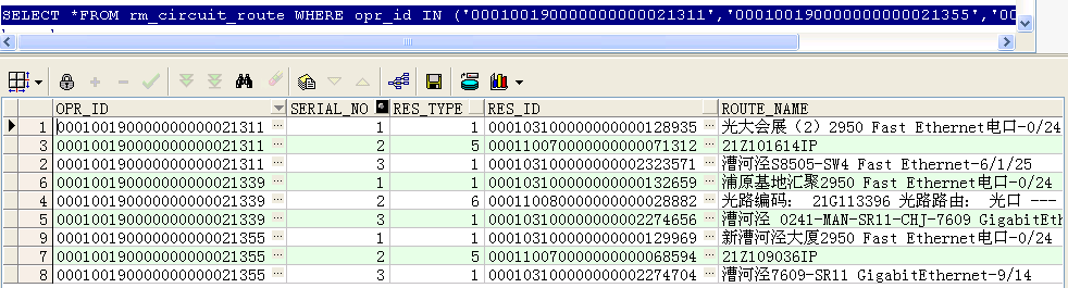
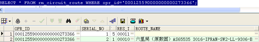
–找出这三条电路每条电路的第一条记录类型和最后一条记录类型

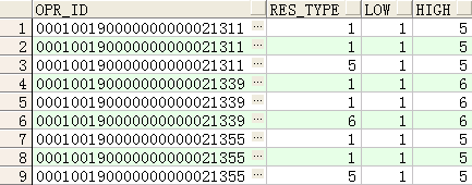
注：rows BETWEEN unbounded preceding AND unbounded following 的使用

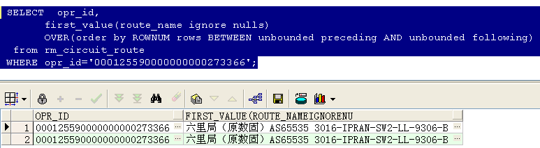
–取last_value时不使用rows BETWEEN unbounded preceding AND unbounded following的结果

数据如下：

取出该电路的第一条记录，加上ignore nulls后，如果第一条是判断的那个字段是空的，则默认取下一条，结果如下所示：

lead(expresstion,<offset>,<default>)
with a as
(select 1 id,’a’ name from dual
union
select 2 id,’b’ name from dual
union
select 3 id,’c’ name from dual
union
select 4 id,’d’ name from dual
union
select 5 id,’e’ name from dual
)
select id,name,lead(id,1,”)over(order by name) from a;

–ratio_to_report(a)函数用法 Ratio_to_report() 括号中就是分子，over() 括号中就是分母
with a as (select 1 a from dual
union all
select 1 a from dual
union  all
select 1 a from dual
union all
select 2 a from dual
union all
select 3 a from dual
union all
select 4 a from dual
union all
select 4 a from dual
union all
select 5 a from dual
)
select a, ratio_to_report(a)over(partition by a) b from a
order by a;

with a as (select 1 a from dual
union all
select 1 a from dual
union  all
select 1 a from dual
union all
select 2 a from dual
union all
select 3 a from dual
union all
select 4 a from dual
union all
select 4 a from dual
union all
select 5 a from dual
)
select a, ratio_to_report(a)over() b from a –分母缺省就是整个占比
order by a;

with a as (select 1 a from dual
union all
select 1 a from dual
union  all
select 1 a from dual
union all
select 2 a from dual
union all
select 3 a from dual
union all
select 4 a from dual
union all
select 4 a from dual
union all
select 5 a from dual
)
select a, ratio_to_report(a)over() b from a
group by a order by a;–分组后的占比

工欲善其事，必先利其器，没有好的工具，怎么能高效的开发出高质量的代码呢？本文为各ASP.NET 开发者介绍一些高效实用的工具，涉及SQL 管理，VS插件，内存管理，诊断工具等，涉及开发过程的各个环节，让开发效率翻倍。